StarAberrationDiagnostics
PixInsight update repository for the StarAberrationDiagnostics script.
This page is informational. For PixInsight, use the repository URL shown below.
Repository URL for PixInsight
https://tricx.de/pi-scripts/StarAberrationDiagnostics/
Installation in PixInsight
- Resources > Updates > Manage Repositories
- Add repository:
https://tricx.de/pi-scripts/StarAberrationDiagnostics/ - Run Check for Updates
- Run via Script > Tricx > StarAberrationDiagnostics
What it does
Diagnoses the optical system from the shapes of the stars across the field:
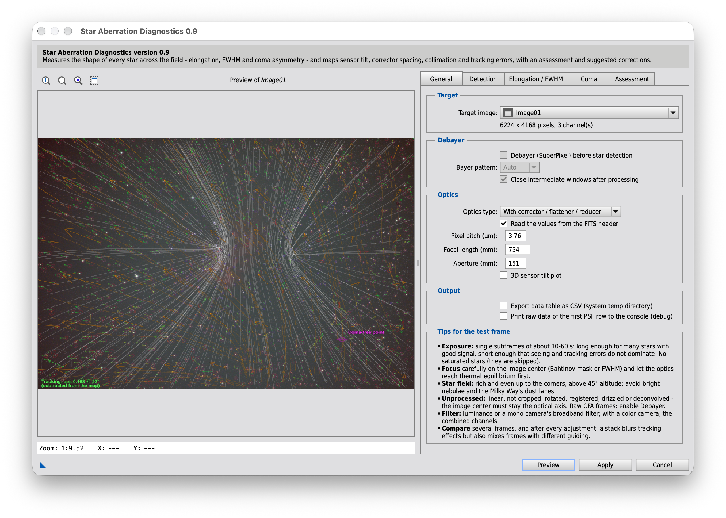
- Vector map of every star's elongation, with streamlines and an orientation heatmap
- Sensor tilt from the FWHM across the field (Siril-style quadrants, 11×11 grid, tilt axis, Δz and tilt angle)
- Corrector spacing and field curvature from the radial/tangential pattern at the field edge
- Coma field and coma-free point from the asymmetry of each star, for collimation
- The tracking error shared by all stars, measured and optionally subtracted
- An assessment of the results with suggested corrections, in the order in which to work through them
- A series analysis of frames before and after a meridian flip, including the plate-solve distortion
- An optional AI review of the results, with a step-by-step explanation
Screenshot
Handbook: how the diagnostics work
The chapters below explain every computation of the script: what each error does to the stars, and how the script captures it mathematically. They build on each other, but each can be read on its own.
- Stars as a probe of the optics
- Finding and measuring the stars
- Describing the shape of a star
- Tracking and guiding errors
- The vector map, streamlines and heatmap
- Focus, sensor tilt and field curvature
- Radial and tangential patterns: corrector spacing
- Coma and collimation
- The assessment and the order of corrections
- Series: before and after the meridian flip
- Plate-solve distortion (SIP)
- The AI review
- Limits and good practice
1.Stars as a probe of the optics
A star is so far away that it is, for all practical purposes, a point. Everything that turns this point into a small disk, an oval or a little comet on the sensor is done on the way: by the atmosphere, the mount, the telescope, a corrector, the camera. The picture a point source makes is called the point spread function (PSF). Because every star in the frame passes through a different part of the optical system, the stars together form a map of how well the optics work at every position of the field.
The script reads this map. For every star it measures four things:
- Size - how far the light is spread, as the full width at half maximum (FWHM).
- Elongation - how much the star deviates from a circle.
- Orientation - in which direction an elongated star points.
- Asymmetry - whether the light leans to one side, like the tail of a comet.
No single star tells much: seeing, noise and neighboring stars disturb each measurement. The strength of the method lies in the pattern over hundreds of stars. A focusing error, a tilted sensor, a wrong corrector distance, a decollimated mirror and a tracking error each leave a pattern of their own, and the chapters below explain which one - and how the script tells them apart.
2.Finding and measuring the stars
Debayering raw color frames
A color camera records a Bayer mosaic: each pixel sees only red, green or blue. An unprocessed mosaic cannot be measured directly - the color pattern would look like structure in every star. The usual debayer methods fill in the missing colors by interpolation, which softens every star a little and in a direction-dependent way. That would falsify exactly what the script measures.
The script therefore uses the SuperPixel method: each 2×2 block (one red, two green, one blue pixel) becomes one color pixel, without any interpolation. The image has half the resolution, and every length converted to micrometers uses the effective pixel pitch of twice the physical pitch.
Detection
PixInsight's StarDetector finds the candidates. If the option Max. stars is set, only
the brightest ones are kept (sorted by flux) - they give the most reliable fits, and the fit is the slow part.
The PSF fit
For every candidate, PixInsight's DynamicPSF fits an elliptical model to the pixels
inside a search box (the search radius). Two models are available. In the coordinates
u, v along the axes of the ellipse (rotated by the angle θ) they read:
The Moffat profile has broader wings than the Gaussian and describes real stars (seeing, diffraction) often better; the Gaussian is faster. From the widths the script computes the FWHM along each axis:
Using the Gaussian factor for a Moffat fit would be a serious mistake: depending on β it would inflate the FWHM by a factor of 1.5 to 2.7 and more.
Quality control
- Detection threshold. A fit counts only above this significance. If not a single star passes, the script lowers the threshold step by step (×0.6, down to 0.2) instead of giving up, and says so.
- MAD outliers. DynamicPSF reports for each fit the mean absolute deviation (MAD) between model and
pixels. Hot pixels, blended pairs or very faint stars produce badly fitting models with a large MAD. A
fit is dropped when
The limit adapts to each frame's noise instead of being a fixed number.MAD > factor · median(MAD of all fits)
- Saturation is checked for the asymmetry measurement (chapter 8): a star whose peak reaches 95% of the full range has a flat top and is skipped there.
3.Describing the shape of a star
The fitted ellipse has a major half axis a (the larger FWHM) and a minor half axis b, and its major axis points in a direction. Three numbers describe how elongated it is - they carry the same information but behave differently in calculations:
The eccentricity colors the vector map. The ellipticity is used wherever a verdict is spoken, because it is easy to read. The distortion is used for averaging and subtracting: only its components add (approximately) linearly when two elongations combine, e.g. an elongation of the optics and one of the tracking.
Direction and the 180° problem
All directions in the script are given in image coordinates: x to the right, y downward, 0° = right, 90° = down. DynamicPSF measures its angle θ counterclockwise on the screen, so the direction of the major axis in image coordinates is ψ = −θ.
An ellipse looks the same when turned by 180°: its orientation is only defined modulo 180°. Averaging the angles directly therefore fails - two almost horizontal stars at 10° and 170° would average to a vertical 90°. The standard remedy, used everywhere in the script, is the double angle: each orientation becomes a vector with the angle 2ψ, the vectors are averaged, and the angle of the mean is halved again.
4.Tracking and guiding errors
The error
If the mount does not follow the sky exactly - periodic error, poor guiding, wind, cable drag, a flexing guide scope - the whole image moves a little during the exposure. Every star is smeared by the same amount in the same direction, regardless of where it is in the field. This is the fingerprint that separates tracking from all optical errors, which vary across the field.
The measurement
The script takes the median of the shape vectors of all stars. The median ignores the minority of stars that are elongated by the optics near the edge and finds what almost all stars have in common:
With the option Subtract it from all stars, this common part is removed from each star before all further analysis - by subtracting the vectors, which is exactly why the distortion χ is used:
Only the shapes are corrected; the star sizes (FWHM) stay as measured. The tracking error would otherwise mask the optical patterns, above all the radial/tangential pattern of chapter 7.
Reading the value
| Common ellipticity | Verdict |
|---|---|
| below 0.03 | OK - tracking is clean |
| 0.03 - 0.07 | Note |
| above 0.07 | Action: check guiding (RMS, calibration), balance, cable drag, wind, flexure |
A direction that stays the same over several frames points to the mount; one that changes points to wind or random guiding errors. The series analysis compares both sides of a meridian flip, where the balance changes.
5.The vector map, streamlines and heatmap
The vector map draws every star as an ellipse at its position, its length and color given by the eccentricity (blue round to red elongated), its direction by ψ. Hundreds of small ellipses are hard to read, so two layers show the large-scale trend.
Streamlines
At any point of the image, the script computes a smoothed orientation from the stars around it: a Gaussian-weighted double-angle mean within a radius R (a percentage of the image diagonal). Nearly round stars have a poorly defined direction, so each star is weighted additionally by the square of its eccentricity:
A streamline follows this field in small steps. Since an orientation has no arrowhead, the script chooses at every step the one of the two directions that continues the previous step - otherwise the line could turn back at random. Streamlines show at a glance whether the stars are aligned radially, concentrically or all in one direction.
Orientation heatmap
The heatmap (after the Seti Astro Suite) fits two smooth polynomial surfaces of a chosen degree over the whole image, one to sin 2θ and one to cos 2θ of all stars, with the coordinates normalized to ±1. Three rounds of 3σ clipping remove outliers. At every point the fitted angle θ = ½ · atan2(s, c) is shown as a hue of a color wheel. A plane (degree 1) can only show a steady gradient; degree 2 and more can follow the curved patterns of coma, but becomes more sensitive to noise near the edges where few stars constrain it.
6.Focus, sensor tilt and field curvature
The physics: blur from defocus
The telescope forms a cone of light that converges to a point in the focal plane. If the sensor sits a distance Δz in front of or behind that plane, it cuts the cone and records a small disk instead of a point. From the geometry of the cone (its opening is the aperture D over the focal length f, i.e. 1/N):
The star in focus is not a point either (seeing, diffraction, optics): it has a size FWHM0. Blurs of independent origin add approximately in quadrature, so the extra blur from defocus follows from the measured FWHM as
This is the bridge from a star size in pixels to a distance in micrometers - and it needs pixel pitch, focal length and aperture, which the script takes from the dialog or the FITS header (XPIXSZ, FOCALLEN, APTDIA or FOCRATIO).
The sign is lost. A disk looks the same whether the sensor is in front of or behind the focus. From one frame, Δz is only a magnitude - which way to turn a tilt screw has to be found by trying (see figure 11).
What the errors look like
- Defocus makes every star larger - but uniformly, so it shows up in the absolute FWHM rather than in its pattern. A telltale sign is a center that is softer than the edge: the focus was set on the edge, or a curved field was focused off the center.
- Sensor tilt makes one side of the frame soft and the opposite side sharp: a one-sided gradient.
- Field curvature makes the edge soft on all sides alike: a symmetric bowl.
Method 1: Siril-style quadrants
Following Siril's "Show tilt", the frame is divided into four quadrants plus an inner circle and an outer ring around the center (radii relative to the half diagonal R). Each area gets the 25%-trimmed mean of the star sizes (FWHMx+FWHMy)/2 - the lowest and highest quarter are discarded before averaging, which makes it robust against single bad fits.
The 11×11 FWHM grid is the same idea at a finer scale: one trimmed mean per cell, noisier but with more detail. The tilt axis is derived from the quadrants. Each quadrant's excess over the center gets a sign, the gradient of a plane through the four values gives the direction of the steepest rise, and with the optics known, its angle:
Per quadrant, the console also lists the defocus Δz = N · √(Fq² − F0²) · p and the angle atan(Δz / distance) to the quadrant center at a quarter of the width and height.
Method 2: the FWHM² surface
Quadrants mix tilt and curvature: a curved field makes all four quadrants soft, a tilt only two. The script therefore fits a smooth surface to the squared FWHM of every star, with X and Y the position relative to the center divided by the half diagonal:
The squares are fitted because blurs add in quadrature (see above): the symmetric term then measures the curvature, the linear terms the tilt, and the two no longer contaminate each other. The fit is a robust least squares fit: four rounds in which stars whose residual exceeds 3 σ (σ from the median absolute residual) are left out. From the coefficients:
A negative c3 means the edge is sharper than the center - the frame is out of focus or was focused on the edge. The script also flags a defocus suspicion when the median FWHM in the inner third (r < ⅓ R) is more than 5% larger than in the outer third (r > ⅔ R). As long as that is the case, tilt and spacing verdicts are unreliable, which is why focus comes first in the suggested order.
The 3D tilt plot
The pseudo-3D plot places the four quadrant values at their physical positions on the sensor (in mm) as signed Δz and fits a plane through the center. Because the sign of Δz is unknown (see the note above), it draws two mirror-image variants. Both are equally plausible; the tilt axis is the same for both.
Verdicts
| Value | OK | Note | Action |
|---|---|---|---|
| Tilt: (FWHMsoft − FWHMsharp) / their mean | < 5% | 5 - 10% | > 10% |
| Field curvature: (FWHMedge − FWHMcenter) / FWHMcenter | ≤ 15% | 15 - 30% | > 30% |
| Focus: defocus suspicion or c3 < 0 | refocus first |
7.Radial and tangential patterns: corrector spacing
The error
A coma corrector, field flattener or reducer is designed for one exact distance to the sensor (the back focus, e.g. 55 mm). At the wrong distance it corrects too little or too much, and the stars at the field edge become elongated - either radially, pointing toward the center like spokes, or tangentially, lying along circles around the center. In an uncorrected system (a bare Newtonian), radial elongation is simply its natural coma.
The measurement
For each star at the position angle φ (seen from the image center), the script measures how much of its elongation lies along the radius:
The stars are grouped into six rings (r/R = 0-⅙, ⅙-⅓, … 5/6-1). Per ring the console lists the number of stars, median FWHM, ellipticity, eps_rad, the radial flare direction asym_rad (chapter 8) and an alignment value between flare and elongation (+1: the flare lies along the elongation, i.e. coma shapes the star). The verdict uses the median eps_rad over the outer third (r > ⅔ R), with at least 10 stars:
| eps_rad (outer third) | Pattern | Rule of thumb of the script |
|---|---|---|
| |eps_rad| ≤ 0.04 | none | OK |
| > +0.04 (action above 0.08) | radial | with a corrector: under-corrected - increase the corrector-sensor distance in small steps (e.g. 0.5 mm); uncorrected system: normal coma |
| < −0.04 (action below −0.08) | tangential | decrease the distance - but defocus combined with field curvature looks the same, so check the focus first |
The direction of the correction is a rule of thumb that holds for many correctors; the manual of your corrector has the final word. Change the distance in small steps and measure again.
8.Coma and collimation
The error
Coma turns stars into small comets: a bright core with a fan of light on one side. In a Newtonian it grows linearly with the distance from the optical axis and points away from it; a coma corrector removes it - or over-corrects it, when it sits at the wrong distance. The point where the coma vanishes marks the optical axis. If the mirrors are decollimated (or a corrector is decentered or tilted), this coma-free point moves away from the image center.
Why the fit cannot see it
Gaussian and Moffat are point-symmetric models: they fit an ellipse around the core and cannot tell on which side the fan sits. The script measures the asymmetry directly on the pixels instead, relative to the fitted center:
- Aperture radius rap = 4σ + 1 px (limited to 3 … 25 px), σ = FWHM/2.3548; background = median of a ring from rap+2 to rap+6 px.
- Weights w = pixel value − background (only positive ones).
- Stars at the border, without a background ring or with a peak at 95% of the range (saturated) are skipped.
The coma field
Third-order coma is linear in the field position. Around the coma-free point P0, the asymmetry vector of a star at position P is therefore modeled as
- k > 0: flares point away from P0 - under-corrected (normal for a bare Newtonian).
- k < 0: flares point toward P0 - over-corrected.
At least 30 stars with a valid asymmetry are needed. The fit is robust (3σ clipping, three rounds). Its uncertainty comes from a bootstrap: the fit is repeated 100 times on random resamples of the stars; the spread of k is its standard deviation, that of P0 a robust spread (MAD), because a few resamples with k ≈ 0 can throw P0 arbitrarily far. The coma counts as significant when |k| > 3 · spread(k). A cross-check fits the same model to the centroid offsets.
Collimation
The script suggests collimating when P0 lies more than 15% of the half diagonal off the center and more than twice its own uncertainty. One caution is built in: an uneven tracking drift adds a constant asymmetry and shifts P0 along the drift. If the offset lies within 20° of the tracking elongation, the suggestion says so - compare several frames before touching the collimation screws.
Coma streamlines
Unlike an orientation, m3 is a true vector with a direction. The coma streamlines follow its Gaussian-smoothed field (at least 8 stars in the radius) with arrowheads, and stop where the field becomes weaker than a set percentage of its strong part - so the coma-free zone does not fake a direction. Under-corrected coma looks like a source, over-corrected coma like a sink.
9.The assessment and the order of corrections
The Assessment tab turns the values of the previous chapters into findings, each judged as OK, Note or Action, with what was found and what to do. Where the direction of a correction depends on the optical system, the Optics type (unknown, uncorrected, with corrector) decides the wording.
The actions are sorted into the order in which they are best worked through, because the errors mask each other:
- Focus - a defocused frame falsifies the tilt and spacing verdicts.
- Tracking - a common elongation hides the radial/tangential pattern and shifts the coma-free point.
- Tilt - a one-sided blur, fixed in the camera connection.
- Collimation - moves the optical axis, around which everything else is measured.
- Spacing - the corrector distance, judged from the edge pattern.
- Coma - strength and sign of the coma field.
- Field curvature - what remains at the edge.
- Data - fewer than 150 stars make all verdicts uncertain.
All thresholds are starting points, not calibrated limits. Seeing, exposure time and the number of stars change what a single frame can tell.
10.Series: before and after the meridian flip
Why a flip helps
A German equatorial mount has to turn the telescope around when the target crosses the meridian. After this meridian flip, the tube is turned by 180° around its axis relative to gravity. Anything that sags or shifts under its own weight - a focuser drawtube, a camera on a long adapter, a primary mirror in its cell ("mirror flop"), a loose corrector - moves to the other side. Anything fixed in the optical train stays as it is.
Comparing frames of both sides therefore answers a question one frame cannot: is an error fixed, or mechanical? A tilt that turns with the side calls for tightening the focuser and the adapters - adjusting the tilt would only fit one side. A tilt that stays calls for the tilt adjustment.
Which side is a frame on?
- Manual - set in the list.
- PIERSIDE - written by N.I.N.A. and most ASCOM/INDI capture programs (West before the meridian, telescope pointing east; East after the flip).
- A camera angle that turns by 180° - e.g. ROTATOR as written by the ASIAIR from its plate solve (also POSANGLE, ANGLE, CROTA2). Frames within 45° of the first angle form one group, those within 45° of the opposite angle the other; the hour angles of their members name the groups.
- The hour angle - from the time, the target's right ascension α and the site longitude λ (east positive):
The comparison
Every frame is measured with the same settings. Per side and value the script takes the median and a robust spread σ = 1.4826 · MAD, which estimates the standard deviation without being fooled by single outliers. The standard error of a median is about 1.253 σ/√n. A value changes at the flip when both hold:
| Value | Practical minimum | A change at the flip means |
|---|---|---|
| FWHM center / edge | 5% | refocusing, temperature or focuser slip |
| Tilt (as a vector: size and direction) | 3 points | sag or play in camera, focuser, adapter |
| Edge elongation eps_rad | 0.02 | play in corrector or drawtube, or a different focus |
| Tracking elongation | 0.02 | balance (east/west heavy), DEC backlash, cable drag |
| Coma k | - | corrector or spacing with play |
| Coma-free point (vector) | 10% of R | mirror flop, loose secondary or corrector |
| Plate-solve distortion (chapter 11) | 1 px | a part of the optics shifts - or a solver convention |
With fewer than 3 frames on a side, there is no verdict. Vectors (tilt, coma-free point, distortion) are compared as vectors: their direction can turn while their length stays.
Drift over the night
Temperature and altitude change slowly, and the frames of one side follow each other in time - a drift can therefore look like a jump at the flip. The script subtracts each side's median and correlates what remains with the time. With at least 6 frames, a correlation |r| ≥ 0.6 and a total change above the practical minimum, the value is reported as drifting, with a warning where it may have faked a change at the flip. If the focuser position (FOCPOS) differs between the sides, the report notes that the frames were refocused.
11.Plate-solve distortion (SIP)
A plate solve finds where every pixel points in the sky. Real optics do not map the sky perfectly onto a flat grid; the SIP convention (Simple Imaging Polynomial) stores the deviation as polynomials in the pixel coordinates u, v relative to a reference pixel:
This measures the positions of the stars - independent of their shapes, and a by-product of every solve. The series analysis reads the six quadratic terms (p + q = 2) from the header. They do not depend on the reference pixel, so they can be compared even when the rest of the solution is missing. The script expresses them as the shift of the four image corners in pixels, and compares these between the sides.
What it can and cannot tell
- No measure of sensor tilt. A tilt θ acts like a slight perspective and shifts a point at the distance r by only about tan θ · r² / fpx (fpx = focal length in pixels). At 750 mm and 4.29 µm pixels, 0.1° moves a corner by 0.07 px - the FWHM method (chapter 6) is far more sensitive. The report shows the tilt a pure perspective would need for the measured terms; a value of several degrees means they have other causes.
- No measure of back focus. The symmetric (pincushion/barrel) distortion of a corrector is a third-order term; many solvers only fit second order.
- A good indicator of movement. If the quadratic terms change at the flip, something in the optical train shifts under gravity - typically the primary mirror of a Newtonian, or a corrector moving in the drawtube. If the coma-free point moves as well, that supports it.
A reversal of sign at the flip can also come from the solver working in a frame that turns with the sky. To be sure, solve one frame per side with PixInsight's ImageSolver and compare. The terms are compared only when all solutions refer to images of the same size.
12.The AI review
On request, the script sends its results to Claude (Anthropic API) for a second opinion - after a Preview, after a series analysis, or both. What is sent:
- the measured values of the chapters above as numbers (tracking, ring profile, FWHM surface and a 5×5 grid, quadrants, coma fit, optics), the rule-based assessment, and optionally the vector map as an image;
- for a series: one row per frame (side, hour angle, altitude, focus, the values above, SIP) and the comparison of the sides.
No image data other than the optional vector map leaves the computer. The answer is forced into a fixed structure: an overall verdict, the order of corrections and, per finding, the measured values it rests on, what the stars look like, the derivation, the alternatives and why they fit less, what to do, how to check it in the next frame, and a confidence with its reason. Step by step explains every technical term for beginners; Short keeps each point to a sentence or two. Requests and answers can be saved as text files next to the frames.
The AI weighs the same numbers the rules use - it can explain and connect them, but it cannot see more than was measured. It needs an Anthropic API key; each request is billed to it.
13.Limits and good practice
- Use unregistered, uncropped frames. Every computation assumes that the image center is the optical axis. Registration, cropping or rotation destroy that.
- Calibrated but unprocessed. Stretching, deconvolution, noise reduction and star reduction change the star profiles.
- Short exposures, good seeing. Seeing and tracking add a blur that hides small optical errors. Several frames give more certainty than one.
- A rich star field - at least 150 measured stars, well spread up to the corners, where the errors are largest.
- One frame cannot tell the sign of a defocus. Where a correction has a direction (tilt, spacing), change it in small steps and measure again.
- Geometric optics. The conversions from blur to Δz ignore diffraction and seeing profiles; they are estimates to guide an adjustment, not measurements with a tolerance.