Dialog reference

StarAberrationDiagnostics measures the shape of every star across the field and turns it into maps and an assessment of the optics. This reference walks through the dialog page by page and explains every setting; how the computations behind it work is explained in the handbook.

The dialog has two halves. On the left is the preview: the tips for the test frames while no image is chosen, the target image before the first Calculate, then the map of the selected Maps tab; on the Assessment and the Series tab, their own results instead (assessments, series hints and report). On the right are the settings in four tabs:

• Setup - the target image, debayering, optics and output (General), and the star detection and PSF fit (Star detection).
• Maps - one sub-tab per map: Size, Shape, Coma and Tilt, each with its layers and its evaluation.
• Assessment - the verdicts with suggested corrections.
• Series - several frames, e.g. before and after the meridian flip, compared.

Typical workflow

1. Open a single, unregistered and uncropped light frame and select it as the target image.
2. Check the optics on Setup › General (or let them be read from the FITS header).
3. Click Calculate. The preview shows the map of the selected Maps tab; switching tabs and layers redraws it at once, without measuring the stars again.
4. Read the Assessment and work through the corrections in the order given.
5. Save opens the maps as image windows (plus CSV and 3D plot, when enabled) and closes the dialog.

Handbook: 2. Stars as a probe of the optics, 13. Limits and good practice

Preview

Zoom buttons

Zoom in, zoom out, 1:1 and zoom to fit. The mouse wheel zooms as well; drag to scroll.

Status line

The zoom factor and the image coordinates under the mouse pointer.

Buttons

New instance (triangle, bottom left)

Drop the current settings as a process icon on the workspace. Double-clicking the dropped icon later reopens the dialog with the same settings.

Note: Dragging directly onto an image is not supported for script processes in current PixInsight versions.

Browse Documentation (book, next to it)

Opens the reference documentation of the dialog in the PixInsight documentation browser.

The documentation is this reference, installed with the script; without the simulators of the maps, which are only on the website.

Calculate

Runs the analysis with the current settings and shows a map in the preview - that of the selected Maps tab (Size, Shape, Coma, Tilt) - without opening a window, exporting the CSV file or drawing the 3D plot. Switching between these tabs switches the map at once. The PSF asymmetry is always measured, so that the coma layers can be switched on later.

After that, the layers and their settings can be changed without measuring the stars again: the preview is redrawn at once. Only a change of the detection settings or the target image needs a new Calculate.

Save

Opens the four maps in new windows: Star size, Star shape, Coma and Tilt (AberrationSize_…, AberrationShape_…, AberrationComa_…, AberrationTilt_…), with the 3D plot and the CSV export when enabled, and closes the dialog. The star measurement of Calculate is reused when its detection settings are still current.

Cancel

Closes the dialog without output. During a computation the button reads Stop and ends it.

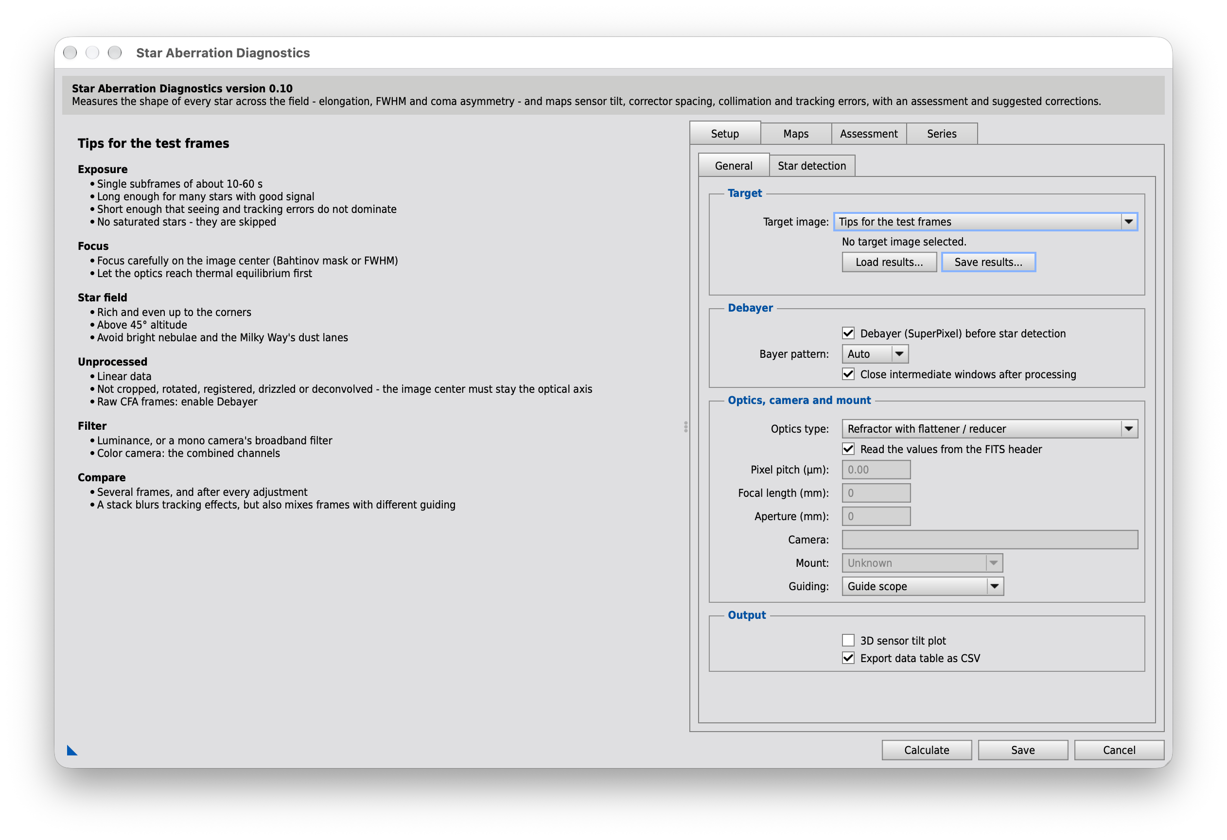
Target

Target image

The image to analyze, from the open image windows. Below it its size and number of channels. Use a single light frame, not registered and not cropped: the image center must be the optical axis.

The last entry, Tips for the test frames, shows instead of an image what makes a good test frame: exposure, focus, star field, unprocessed data, filter and comparing several frames. The same tips appear while no image is open.

Load results…

Loads results saved with Save results and shows them as after a Calculate, without measuring the stars again: the maps, their evaluations, the assessment and Save all work with them. Optics, mount and observation values come from the saved FITS header (or the fields above), the layers from the current settings.

The background is the image when it is open (same view and file), else dark. The detection settings of the dialog do not apply to loaded results; the next Calculate measures the target image again.

Save results…

Saves the stars measured by the last Calculate (or loaded results) as a file name_aberration.json, by default next to the image: positions, FWHM, shape and asymmetry of every star, the detection settings and the FITS header of the image - about 100 bytes per star. The maps, the evaluations and the assessment are computed from it again on loading; the current layer and optics settings are not part of it.

Loaded results

While loaded results are shown, a line below the buttons names the file and its number of stars.

Debayer

Debayer (SuperPixel) before star detection

Creates a debayered copy of the target image (SuperPixel method: direct 2x2 pixel grouping without interpolation, half resolution) and continues working on this copy. The original image is left unchanged. Only enable this if the target image is still an unprocessed Bayer mosaic (not true RGB).

It also applies to the frames of the Series tab. It is disabled for a color target image unless the Series tab lists frames; color images are never debayered.

Leave it off for a monochrome camera and for an image that is already RGB. Debayering it yourself with VNG or bilinear interpolation works too, but broadens the star profiles slightly.

Bayer pattern

• Auto
• RGGB
• BGGR
• GBRG
• GRBG

'Auto' reads the Bayer pattern from the image's FITS/RAW metadata. If that fails ('Unable to acquire CFA pattern information'), manually select the actual sensor pattern here (see the camera specification).

Close intermediate windows after processing

Closes the debayered SuperPixel intermediate window as well as any side windows created during the debayer step (e.g. noise evaluation) once the vector map has finished drawing. Only relevant if debayering is enabled.

Optics, camera and mount

Optics type

• Unknown
• Reflector without corrector (e.g. bare Newtonian)
• Reflector with coma corrector / reducer
• Refractor without flattener
• Refractor with flattener / reducer
• RASA / Hyperstar (f/2)
• SCT with reducer (e.g. f/6.3)
• Aplanatic SCT (EdgeHD and similar)
• Classic SCT or Maksutov (no corrector)
• Astrograph with built-in flattener (Petzval, quadruplet)

The optical system, for the suggestions of the Assessment page. A bare Newtonian shows coma and field curvature by design; with a coma corrector, field flattener or reducer, the same patterns point to its spacing. A refractor has hardly any coma: without a flattener, field curvature and astigmatism at the edge are expected, and its lens is collimated at the factory. In a color or broadband frame, a refractor's lateral color elongates the edge stars radially like under-correction. With Unknown, the suggestions name both cases.

SCT, Maksutov and RASA focus by moving the primary mirror (mirror flop). A classic SCT has coma and a curved field by design; a Maksutov or SCT at f/10-f/15 is seeing-limited with a deep focus zone, so small differences across the field are uncertain. An aplanatic SCT (EdgeHD), a RASA and an astrograph with built-in flattener are meant to be flat: curvature and coma point to the back focus. A RASA at f/2 reacts to a few micrometers of tilt.

Read the values from the FITS header

Uses XPIXSZ (pixel pitch, by convention including binning), FOCALLEN and APTDIA (or FOCALLEN/FOCRATIO) from the target image's FITS header (and from each frame's header in a series). The fields below then show these values, read-only; a value the header does not give is not set (0) - without an image, all three. Uncheck to enter your own values instead: they are saved and used for every image. Always the physical sensor pitch - the doubling after SuperPixel debayering is applied automatically.

Pixel pitch (µm)

Physical pixel size of the sensor in micrometers (e.g. 4.31 for a Canon EOS 550D). 0 = not specified, the tilt angle computation is then skipped. Always enter the physical sensor pitch - with SuperPixel debayering the script automatically uses twice this value (one output pixel = 2x2 sensor pixels).

Grayed: "Read the values from the FITS header" is checked - the value comes from the header of the target image (XPIXSZ), 0 when it has none or there is no image. Uncheck it to enter your own value, which is saved.

Focal length (mm)

Focal length of the telescope in mm (e.g. 750 for a Skywatcher 150P).

Grayed: from the FITS header of the target image (FOCALLEN), 0 when it has none.

Aperture (mm)

Aperture of the telescope in mm (e.g. 150 for a Skywatcher 150P). Together with the focal length, this gives the f-number (focal length/aperture).

Grayed: from the FITS header of the target image (APTDIA, or FOCALLEN/FOCRATIO), 0 when it has none.

Camera

From the FITS header of the target image (INSTRUME, binning from XBINNING/YBINNING), when "Read the values from the FITS header" is checked. For information only.

Mount

• Unknown
• German equatorial (GEM)
• Equatorial fork
• Alt-azimuth, tracked
• Not tracked

The mount, for the assessment: an alt-azimuth mount without a derotator turns the field during the exposure - the stars become arcs around the rotation center, a tangential pattern like field curvature; the assessment then gives its size at the corners (from EXPTIME, CENTALT, CENTAZ and SITELAT) and warns.

With "Read the values from the FITS header" it is estimated (grayed, the source beside it): PIERSIDE East/West means a German equatorial mount; otherwise the mount driver's name in TELESCOP (EQMod, GS Server, iOptron CEM, AM5 … equatorial; Alt-Az, AZ-GTi, Seestar, Dwarf … alt-azimuth); else unknown. Uncheck it to choose the mount yourself.

Guiding

• Unknown
• Not guided
• Guide scope
• Off-axis guider (OAG)
• Guided, method unknown

How the exposures were guided - it decides what a common elongation of all stars means:

Not guided: the mount's tracking (periodic error of the worm, polar drift).

Guide scope: differential flexure between guide scope and main optics or mirror flop when it is the same in every frame, the guiding quality when it changes.

Off-axis guider: no differential flexure - the same in every frame points rather to astigmatism on the axis.

No FITS keyword says this; it is saved, also with "Read the values from the FITS header". With Unknown, a guide camera in the header (GUIDECAM, written by the ASIAIR) counts as "guided, method unknown" - shown beside the field.

Output

3D sensor tilt plot

Opens a separate window with an isometric 2D graphic (PJSR has no true 3D): a flat reference plane next to the tilted plane computed from the Δz values. Created by Save (and per frame by a series). It needs pixel pitch, focal length and aperture - from the image's FITS header or the fields above: an image without them is skipped with a console note.

Export data table as CSV

Save: name_aberration.csv next to the original file (the temporary directory for an image that was never saved). Analyze series: StarAberrationSeries.csv in the directory of the frames. Existing files are replaced.

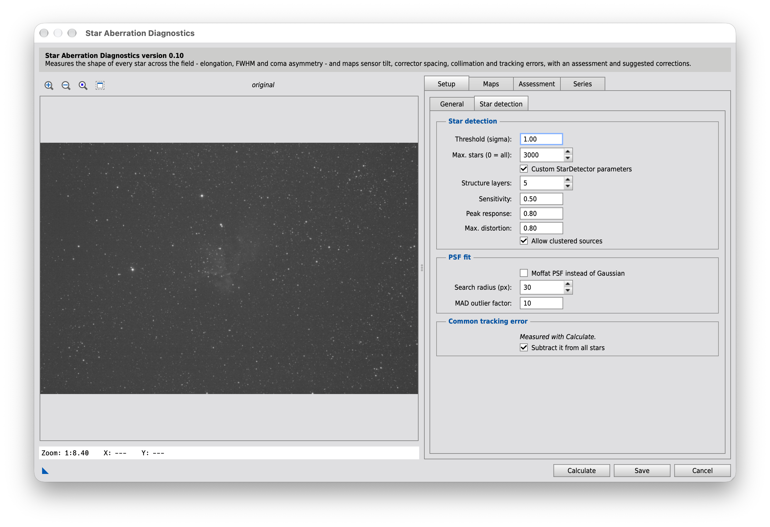
Star detection

Threshold (sigma)

Star detection threshold in units of the background noise. Lower = more, but possibly less reliable stars.

Max. stars (0 = all)

Limits the number of candidates passed to DynamicPSF to the N brightest (sorted by StarDetector flux). The PSF fit is a single, blocking call with no visible intermediate progress - fewer candidates directly shorten its runtime. 0 = fit all found candidates.

Custom StarDetector parameters

Off: StarDetector runs with its own defaults (structure layers 5, sensitivity 0.5, peak response 0.5, max. distortion 0.6, no clustered sources). These reject strongly elongated and large stars - exactly the aberrated stars at the field edge, which then leave the corners of the FWHM grid empty or sparsely populated.

On: the values below are used.

The four fields and the checkbox below are only used while this is checked.

Structure layers

Number of dyadic wavelet layers: the largest detectable structure is about 2^n pixels (5 = 32 px). Increase it for large, defocused or strongly aberrated stars. Default 5.

Sensitivity

0..1, higher = fainter stars are detected. Default 0.5.

Peak response

0..1, higher = more tolerant of flat star profiles (bloated stars at the field edge); lower = only stars with a prominent peak. Default 0.5.

Max. distortion

0..1, higher = more elongated or irregular stars are accepted. Raise it (e.g. 0.8) when the stars at the field edge are strongly elongated. Too high also lets galaxies and blends through. Default 0.6.

Allow clustered sources

Detect non-separable double/multiple stars as single objects. Their centroids and shapes are unreliable, so this is off by default.

PSF fit

Moffat PSF instead of Gaussian

Moffat is the more realistic profile for stars with a diffraction disk, Gaussian is faster.

Search radius (px)

Search radius of the PSF fit in pixels; adjust to the star size.

MAD outlier factor

Rejects PSF fits whose MAD (mean deviation from the model) is more than X times the median of all successful fits in this image. Filters out noisy/unstable fits (hot pixels, blends, very faint candidates) that would otherwise show up in the vector map as physically implausible, isolated outliers (strong eccentricity right next to calm neighboring stars). 0 = filter disabled.

Common tracking error

Measured tracking error

The median elongation of all stars: ellipticity, eccentricity and the direction of the major axis (image coordinates: 0° = right, 90° = down). Below an ellipticity of 0.03 it is negligible.

Shows Measured with Calculate until the first Calculate, then the measured value.

Subtract it from all stars

Optical aberrations form patterns that are symmetric around the optical axis and average out over the field; an elongation shared by all stars comes from tracking/guiding, wind or flexure. Its median is always reported in the console; with this option it is also subtracted from every star before the vector map, streamlines, heatmap and the ring analysis are computed, so the optical pattern is not masked by the mount. The CSV keeps the raw values in extra columns.

Above all map tabs

Show

• Target image (Calculate)
• Series static: group (n frames)

Target image (Calculate): the image measured by Calculate - to check the settings on one frame before running a series.

Series static: after Analyze series, the stars of all frames (or of one side of the flip) pooled. Each frame loses its dynamic tracking (its own uniform term less the mean of the group) and its FWHM is scaled to the median center FWHM, so the seeing drops out: what remains is fixed to the sensor - the optics, plus any constant tracking, which a single camera angle cannot tell from astigmatism on the axis. With n frames the standard errors are about √n smaller. The background is dark: the pooled stars belong to no single frame.

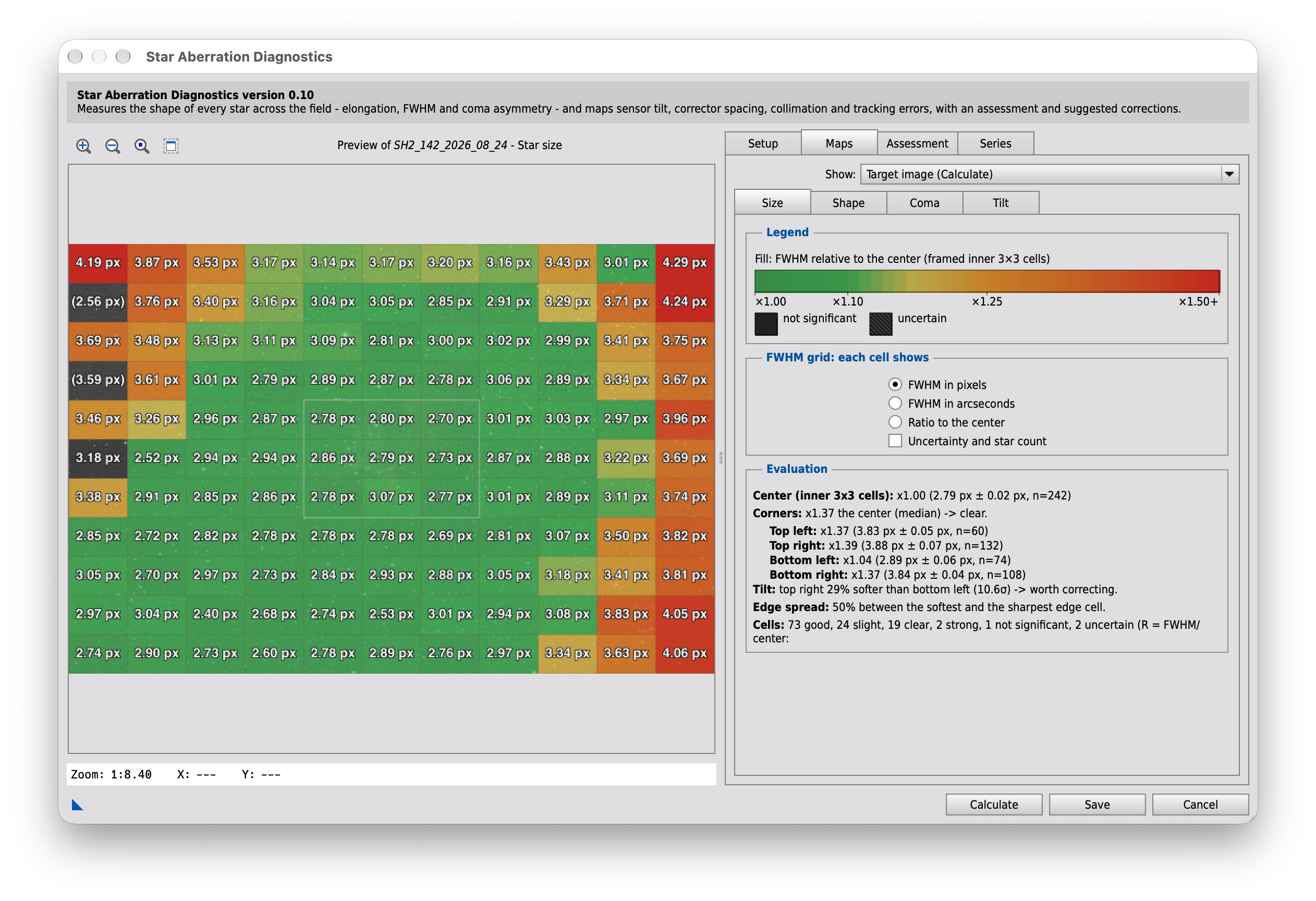
Legend

Fill colors

The 11×11 grid shows per cell its FWHM (25%-trimmed mean) in pixels and/or arcseconds and its ratio to the center (inner 3×3 cells): ×1.17 = 17% larger stars than in the center. The fill follows the ratio and its class: green ≤ 1.10 good (as sharp as the center, or sharper), yellow slight, orange clear (around 1.25), red ≥ 1.50 strong - only where the cell differs from the center by at least 2σ (or is good anyway); an unfilled cell cannot be told from the center.

Hatched, value in (brackets): uncertain - fewer than 5 stars, or a standard error above 10% of the value.

The Evaluation box gives the center FWHM, the corners (median ratio of the 2×2 corner blocks: field curvature / spacing) and the tilt (relative difference of the more unequal diagonal, with its significance: < 5% unremarkable, 5-10% slight, > 10% worth correcting). The console lists the details. Each cell has only a fraction of the stars: the tilt axis and the tilt angles use the 4 quadrants.

Green or not significant? Green means the cell is at most 10% larger than the center - good, whatever the noise. Not significant (unfilled) means the cell looks more than 10% larger, but the difference to the center is less than 2σ: a deterioration is not proven there, nor ruled out.

Uncertain or not significant? Uncertain (hatched) means the cell itself is not measured well enough - fewer than 5 stars or a standard error above 10% - and is not judged at all. Not significant means the cell is measured well, but its difference to the center is within the noise.

FWHM grid: each cell shows

FWHM in pixels

Each cell shows its FWHM in image pixels (3.15 px).

FWHM in arcseconds

Each cell shows its FWHM in arcseconds (2.07"), using 206.265 × pixel pitch [µm] / focal length [mm]. Needs pixel pitch and focal length (Setup › General; with SuperPixel debayering, twice the pitch is used automatically) - pixels otherwise.

Ratio to the center

Each cell shows its FWHM relative to the center (inner 3×3 cells): ×1.17 = 17% larger stars than in the center - the value the fill and the assessment are based on.

Uncertainty and star count

Adds a smaller line to every cell: ± the 1σ uncertainty of its FWHM (its standard error, 1.4826 × MAD / √n - not the scatter of the stars; in pixels, or in arcseconds when only those are shown) and n = number of stars. Two cells differ reliably only when their difference exceeds about 2-3 × √(σ₁² + σ₂²).

Evaluation

Evaluation

After Calculate: the center FWHM, the cell counts per class, the corners (field curvature / spacing), the tilt along the more unequal diagonal and the spread of the outer ring.

Simulator

The simulator draws the map for an image of random stars whose size follows a simple optical model, and evaluates it like the script. Set the corrector spacing and the sensor tilt and watch how field curvature, tilt and focus show up in the cells and in the Evaluation box - and how many stars it takes to tell them from the noise.

Errors

Optics and sensor

Measurement and display

The section below the map shows, along both diagonals, where the stars are focused (the image shell) and where the sensor is; the gap between them is the defocus Δz of the stars there. The true values above it come straight from the model; the map and the Evaluation box see only the measured stars, with their scatter and the trimmed mean of the script. The true values hold for the outermost point of each corner; the script pools the 2×2 corner cells, whose stars lie on average closer to the center, so it measures smaller ratios there.

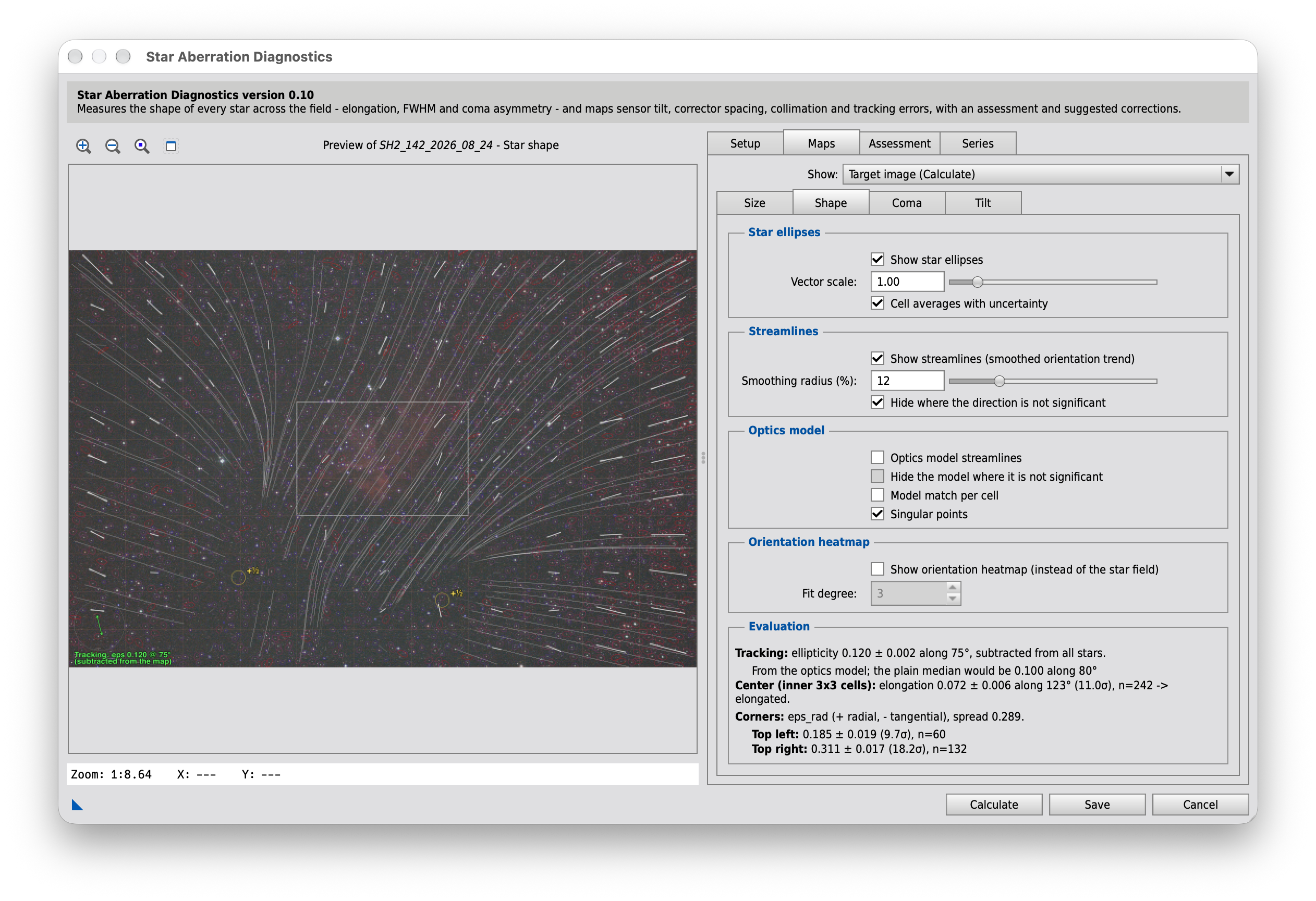
Star ellipses

Show star ellipses

Draws the fitted ellipse of every star. Uncheck to look at the streamlines or the orientation heatmap alone.

Vector scale

Size of the star ellipses here and of the arrows on the Coma map - purely visual.

Cell averages with uncertainty

One bar per cell of the 11×11 grid along the mean axis of its stars (averaged in the doubled angle, since an axis has no direction), its length the mean elongation. The white fan shows the uncertainty of the axis (± standard error / (2 × elongation)). Bright with fan: significantly elongated (≥ 2.45σ); thin and gray: round within the noise; gray dot: fewer than 5 stars.

Streamlines

Show streamlines (smoothed orientation trend)

Shows the large-scale trend of the PSF orientation as continuous lines (like field lines), smoothed over neighboring stars. Radial pattern = under-corrected coma (corrector too close), concentric pattern = over-correction, defocus or field curvature, a pattern that differs between the two sides = tilt; all field lines parallel = tracking. Easier to spot than the noisy per-star vector map alone. Correctly accounts for the fact that the PSF orientation is only defined mod 180° (double-angle averaging).

White: the direction is significant there; gray: it is not (see the option below).

Smoothing radius (%)

How far neighboring stars contribute to smoothing the orientation field, in % of the image diagonal. Smaller = follows local detail more closely (noisier), larger = smoother, more large-scale trend.

Hide where the direction is not significant

The streamlines show only a direction, never its strength: on pure noise they still look orderly. They are therefore white where the smoothed elongation is at least 2.45 times its standard error (the local scatter of the stars over their effective number; pure noise exceeds that in 5% of the places) and gray elsewhere. With this option the gray parts are left out.

Optics model

Optics model streamlines

Fits what optics can produce to all stars: a uniform term (tracking residue, astigmatism on the axis), linear terms (a decentered pattern, binodal astigmatism of a misaligned system) and a radial/tangential term growing with r² (field curvature, corrector spacing). Draws its streamlines in violet (muted where it is not significant); "Model match per cell" below shows where the stars agree with it. The Evaluation below gives how much of the pattern it explains and its residual chi²/dof (about 1 = explained down to the noise).

Hide the model where it is not significant

The model lines are violet where the model's field is at least 2.45 times its standard error (from the uncertainty of the 7 fitted terms), and a muted gray-violet where it is not - near the points where its terms cancel, and wherever the stars do not pin it down. With this option the muted parts are left out.

Model match per cell

Compares each cell with the optics model: the mean difference between the stars' shapes and what the model predicts there, in units of its standard error (scatter of the stars / √n).

Magenta: 3σ or more - the cell holds structure no optics of the model produce (bent or pinched optics, dew, vignetting by an off-axis guider or the focuser, nebulosity, halos, double stars - or a pattern of higher order than the model). About one magenta cell per frame is chance; the Evaluation gives the expected number.

Green: less than 3σ - the cell agrees with the model within its noise.

No frame: fewer than 5 stars.

Singular points

Marks the points where the smoothed axis field has no direction, with their index: optics produce at most one +1 (radial or tangential pattern around the axis) or two +½ (the same split by a uniform term, or binodal astigmatism). More points, and any −½, are noise in the smoothed field - a larger smoothing radius or more stars help.

Orientation heatmap

Show orientation heatmap (instead of the star field)

Replaces the image background with a color-field heatmap of the PSF orientation (like the Seti Astro Suite's "Orientation Map", github.com/setiastro/setiastrosuite): θ is fitted per double-angle averaging (with 3-sigma clipping) as a smooth 2D polynomial surface over all stars (degree set below) and colored as the hue of an HSV color wheel - color gradients show the large-scale orientation trend (tilt/coma) more directly than the real star field. Requires enough stars for the chosen fit degree, otherwise it automatically falls back to the normal background.

Fit degree

Degree of the 2D polynomial fitted to the star orientations. 1 = a plane (pure, uniform tilt only - matches the Seti Astro Suite's default). 2 or higher lets the heatmap also follow local curvature (e.g. a coma pattern) that a plane cannot represent and that may otherwise only show up in the streamlines overlay - at the cost of being more sensitive to noise/outliers, especially near the image edges where fewer stars constrain the higher-order terms.

Evaluation

Evaluation

After Calculate: the elongated and round cells, the significance of the pattern, and how much of it the optics model explains.

Simulator

The simulator draws the map for an image of random stars whose shapes follow a simple optical model, and evaluates it like the script. Set the corrector spacing, the sensor tilt, tracking and collimation and watch which pattern each of them leaves in the ellipses, the streamlines and the Evaluation box - and how the optics model tells them apart.

Errors

Optics and sensor

Measurement

Display

The true values below the Evaluation box come straight from the model, without noise; the map and the Evaluation box see only the measured stars. The true values hold for the outermost point of each corner; the script pools the 2×2 corner cells, whose stars lie on average closer to the center, so it measures smaller values there. Worth trying: a spacing error of either sign (radial or tangential edge), a tilt without spacing error (radial on one side, tangential on the other - a pattern the optics model cannot explain), a focus offset (the whole edge radial or tangential, like a spacing error), tracking with and without Subtract it from all stars, and an optical axis off the center (the axis of the pattern moves with it).

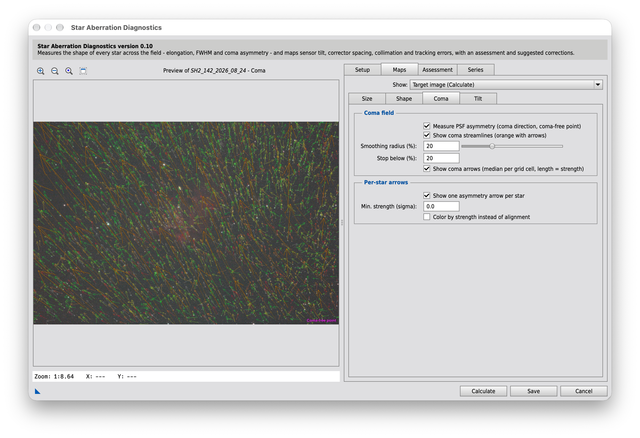
Coma field

Measure PSF asymmetry (coma direction, coma-free point)

Gaussian/Moffat fits are point-symmetric and cannot show on which side of the core a comatic flare sits. This option measures the flux centroid and the third moment of each star directly on the pixels relative to the PSF-fit center, draws the median flare direction on a coarse grid (orange arrows), fits the coma field v = k·(P − P0) and marks the coma-free point P0 (magenta) with its bootstrap uncertainty. Adds a few seconds of runtime.

Show coma streamlines (orange with arrows)

Streamlines through the smoothed PSF-asymmetry field (flare direction) instead of the ellipse orientation. Unlike the elongation streamlines they have a real direction (arrowheads) and stop where the coma becomes weak. Under-corrected coma: lines diverge from the coma-free point (source); over-corrected: they converge on it (sink). Deviations from straight radial lines show what a simple coma model cannot, e.g. a tilted corrector. Requires "Measure PSF asymmetry".

Smoothing radius (%)

Smoothing radius of the asymmetry field, in % of the image diagonal. The per-star asymmetry is much noisier than the ellipse orientation, so this radius should be larger than the one for the elongation streamlines (default: about twice).

Stop below (%)

A line ends where the smoothed asymmetry drops below this percentage of the field's strength (90th percentile over the seed points). Higher = only the clearly comatic regions, lower = lines reach further into the coma-free zone (noisier).

Show coma arrows (median per grid cell, length = strength)

Orange arrows on a 9×6 grid with the median flare direction per cell. Unlike the streamlines, their length shows the strength directly. Requires "Measure PSF asymmetry".

Per-star arrows

Show one asymmetry arrow per star

Draws the measured flare direction of every star as an arrow from the star center (length = strength, scaled with the vector scale), for a star-by-star comparison with the ellipses. Default color: alignment with the ellipse axis - green = parallel (coma shapes the star), red = perpendicular (elongation from defocus/field curvature/astigmatism), gray = star nearly round. Arrows below the threshold are hidden. Requires "Measure PSF asymmetry".

Min. strength (sigma)

The per-star asymmetry is noisy. Its noise is estimated from the inner field, where the coma is close to zero; only arrows stronger than this many sigma are drawn. 0 = draw all.

Color by strength instead of alignment

Colors the per-star arrows by their strength instead of their alignment with the ellipse axis.

Simulator

The simulator draws the map for an image of random comatic stars and evaluates it like the script. Set the residual coma of the corrector and a decollimation and watch the arrows, the streamlines and the coma-free point - and what the console reports.

Optics

Measurement

Display

Below the map are the lines the script writes to the console, and below them the true values of the model; the dashed cyan circle marks the true coma-free point, the magenta cross the fitted one. Worth trying: the residual coma from 1 (no corrector) through 0 (matching corrector) to negative values (over-corrected, the arrows point inward); a decollimation without corrector (the coma-free point moves by the decollimation divided by the residual coma, so a small residual moves it far); and a well-corrected system with much noise, where the coma-free point can no longer be determined. In the model the third moment grows more slowly than the coma itself where the coma is strong; the linear field model of the script then puts the coma-free point a little off the true one - further than its bootstrap uncertainty says.

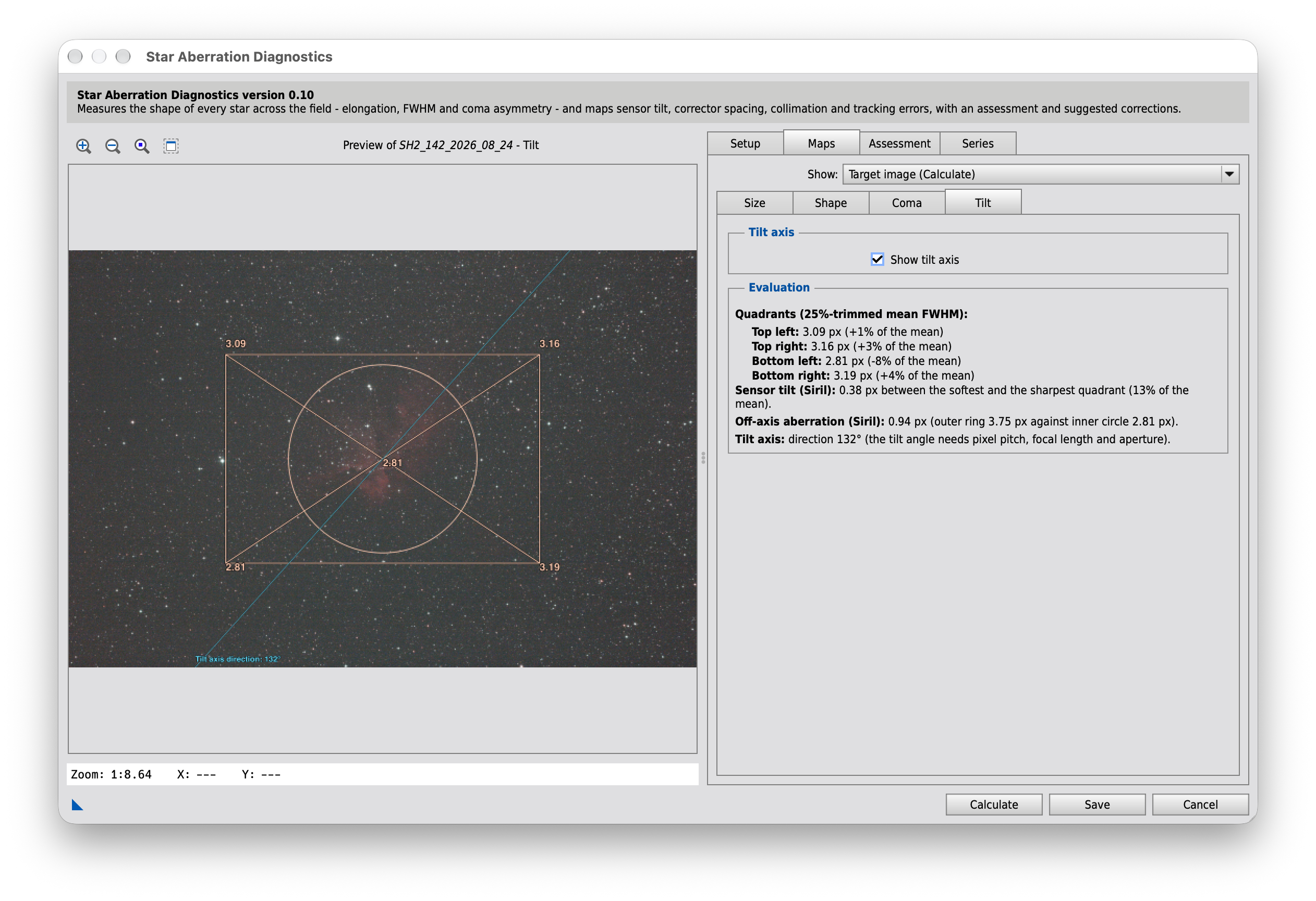
Tilt axis

Show tilt axis

Draws the light-blue tilt axis through the sensor center, derived from the 4-quadrant FWHM evaluation, with its angle/direction label.

Reading the map

The yellow quadrilateral is recreated from Siril's "Show tilt" (ccd-inspector.c): one corner point per image quadrant, its distance from the center proportional to the deviation of that quadrant's mean FWHM from the average of all four. Coarser than the 11×11 grid of Star size, but each quadrant has a quarter of all stars. The light-blue tilt axis runs through the sensor center along the steepest rise of the plane through the four quadrants.

Evaluation

Evaluation

After Calculate: the FWHM of the four quadrants, the tilt and - with pixel pitch, focal length and aperture - Δz and the tilt angle.

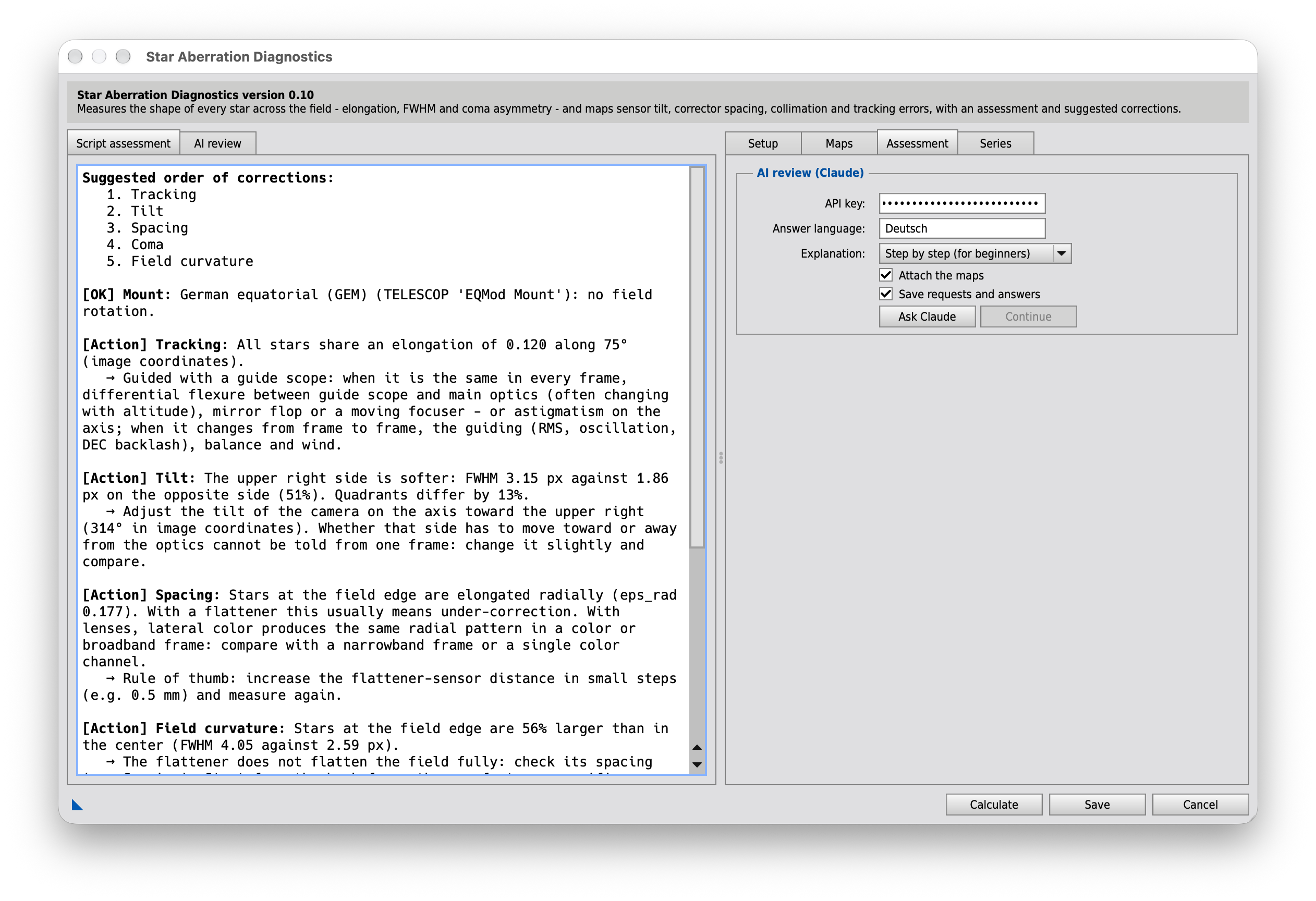
Left side: the assessment

Script assessment

Filled by Calculate. It begins with the suggested order of corrections, followed by one entry per topic (data, mount, focus, tracking, tilt, spacing, coma, field curvature …) with its verdict - [OK], [Note] or [Action] - and, where something is to be done, a suggestion after an arrow. The settings of Setup › General - optics type, mount and guiding - shape the suggestions.

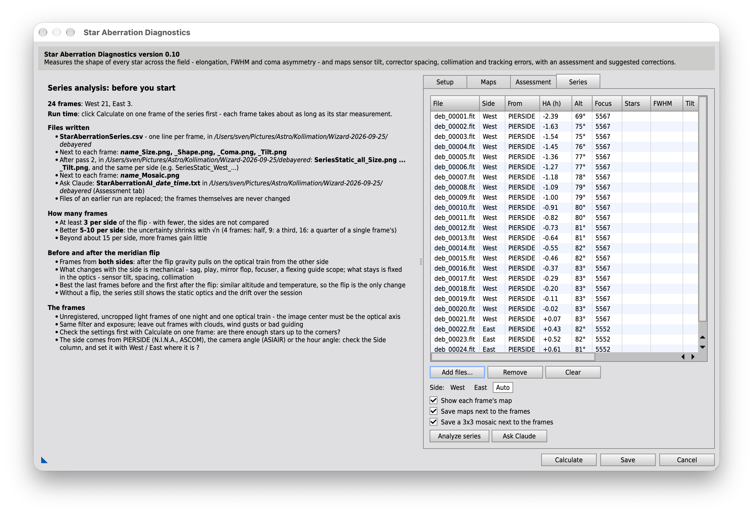
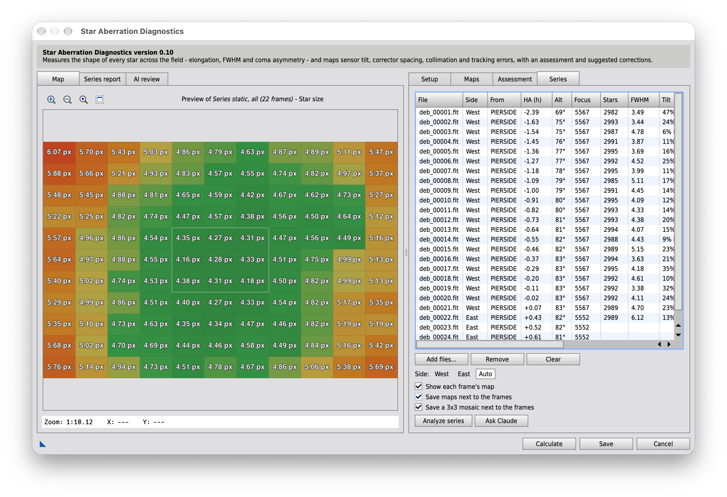
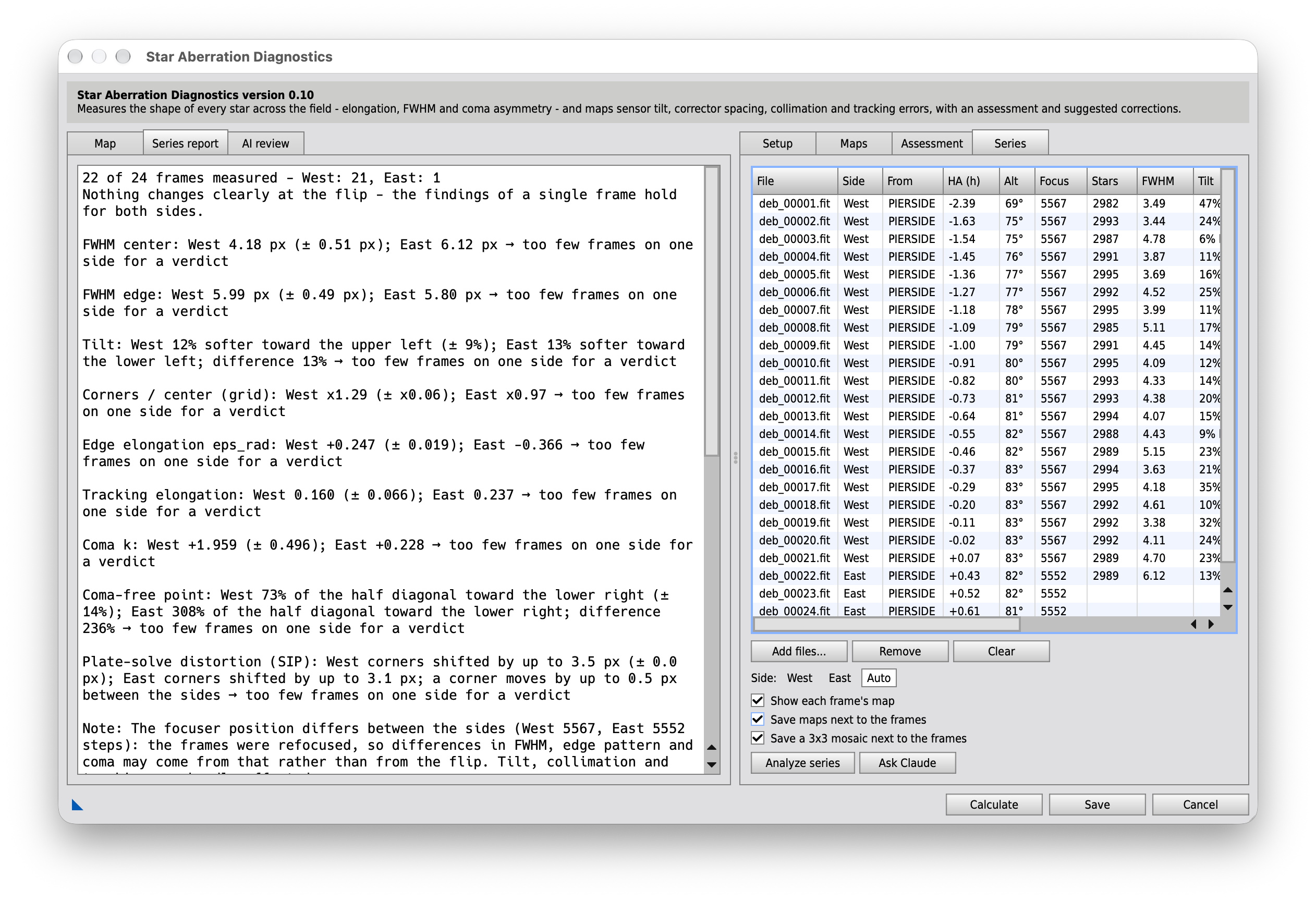
Left side

Hints before a run

Shown until the first Analyze series: the frames listed so far with their sides and an estimate of the run time, the files a run will write with the current settings (CSV table, maps, mosaics - the frames themselves are never changed), and tips on how many frames to take, on frames before and after the meridian flip and on the frames themselves.

Map

The map of the series: during the run each frame's map as soon as it is measured (with Show each frame's map), afterwards the static result of all frames (Maps - Show: Series static). Clicking a frame in the list shows its map again.

Series report

The comparison of the frames and sides after Analyze series. It is shown as soon as the frames are measured; the static result of pass 2 follows below. After a Stop, its first lines say after which frame the run ended and how many frames were not measured; pass 2 is then skipped. The console also names a frame whose header could not be read and that was skipped.

Frames

Frame list

The light frames of the series. From tells where the side comes from: the PIERSIDE keyword (N.I.N.A., ASCOM), a camera angle that turns by 180° at the flip (ROTATOR of the ASIAIR), the hour angle, or manual. Frames close after the meridian may have no known side.

Use unregistered, uncropped frames: the image center must be the optical axis.

Add files…

Adds light frames (FITS or XISF) to the list.

Remove

Removes the selected frames from the list.

Clear

Empties the list.

Side

Sets the side of the selected frames.

West

Before the flip: telescope west of the pier, pointing east (as N.I.N.A. writes PIERSIDE).

East

After the flip: telescope east of the pier, pointing west.

Auto

Takes the side from the header again (PIERSIDE, camera angle or hour angle).

Maps

Show each frame's map

Draws the map of the selected tab (Star shape, Star size or Coma) of each frame in the preview as soon as it is measured, and keeps a reduced copy: clicking a frame in the list shows it again. This takes a few seconds more per frame.

Only the display changes: the analysis of Calculate and the Assessment tab stay as they are.

Save maps next to the frames

Saves for each frame the images Save opens, as PNG in the frame's directory, named after the frame so that they sort right after it:

name_Size.png, name_Shape.png, name_Coma.png, name_Tilt.png - the four maps with the layers of their tabs

name_Aberration3D.png - the 3D sensor tilt plot, when it is enabled (Setup > General) and pixel pitch, focal length and aperture are known

After pass 2 also SeriesStatic_group_Size.png … _Tilt.png in the directory of the first frame - the static maps of all frames and of each side.

Files of an earlier run are replaced.

Save a 3x3 mosaic next to the frames

Saves for each frame a mosaic as AberrationInspector draws it: the four corners, the four edge centers and the image center, each cropped 1:1 to 512 x 512 px of the stretched image, separated by gray lines.

name_Mosaic.png - PNG, in the frame's directory

With Debayer enabled, the tiles come from the half-size SuperPixel image. Files of an earlier run are replaced.

Run

Analyze series

Measures every frame with the current settings (Setup > Star detection, debayer, tracking subtraction, optics) and compares the sides: tilt, FWHM, edge pattern, tracking, coma strength and coma-free point, each judged as stable or changing at the flip, plus drifts over the session.

Each frame takes about as long as a Calculate. Stop ends the run after the current frame; the frames measured so far are compared, pass 2 is skipped. The CSV export (Setup > General) writes one line per frame.

Pass 2 then pools the stars of all frames, and of each side, after taking out each frame's dynamic tracking (its own uniform term less the mean) and scaling its FWHM to the median center FWHM: the static optics with about √n smaller errors. The maps show it at once (Maps - Show: Series static); the report gives the static and the dynamic tracking. Calculate stays a single pass on the target image - to check the settings before a series.